Facial Recognition in Python - James Barnden Blog

Check it out on GitHub

Follow @JBarnden Star Watch Fork Download

In this series of articles, I’ll be giving an overview of what a facial recognition pipeline might be composed of, some different approaches (both supervised and unsupervised), and how to implement and evaluate them in Python. This series of articles assumes you’re somewhat familiar with python, and are somewhere between beginner and intermediate in the world of machine learning.

By the end of this article, we’ll have broadly covered all the steps of a generic facial recognition system/pipeline, and will have put together and trained a supervised facial recognition system in Python. Sound cool? Read on!

Note: You’ll find the python notebook containing the full tutorial code in the Links and Resources section

Pipeline Overview
Supervised Facial Recognition in Python
Loading the Dataset
Training and Testing the Recognizer
Conclusion
Links and Resources

A Generic Facial Recognition Pipeline

There are four stages in a general facial recognition pipieline, these are:

Facial detection – Finding individual faces in an image, cropping and saving these as separate images which we’ll call raw faces.
Feature extraction – Processing/compressing raw faces to reduce unwanted “noise”, and make the images more digestible for our machine learning algorithms. This results in a set of feature vectors, one for each of the faces we found.
Feature comparison – Looking at our feature vectors to identify similarities and dissimilarities that can help tell different people apart. This results in a model, which we can use for reference when trying to recognize new images of faces that our system hasn’t seen before.
Recognition – We can present new unseen raw faces to the system, put them through the feature extraction process, and use the model to attempt to recognize who the face belongs to (or assign a label from our model to the face).

If this seems a bit fuzzy now, it’ll become clearer when we get in to some code. While these are the steps of a facial recognition system, it should be noted here that there are several different ways of doing each of these steps, all with their own advantages and disadvantages, that are all applicable for different situations and scenarios. Our ideal goal is to be able to recognize the features of one persons face under a variety of conditions. While we may have several pictures of Steve, what happens when the lighting is different, or when he turns his head, opens his mouth, or blinks in a picture? Some methods of feature extraction can be quite susceptible to these things, which can result in a big difference between feature vectors. As a simplified example if we ask an algorithm to compare the words “Tree” and “tree”, while we know they’re the same word, the algorithm will tell us they’re different (capitol T and lowercase t) unless we process the words properly first (make everything lowercase consistently). This is essentially the same problem, and something we’ll explore in greater depth in future articles.

If you’re somewhat familiar with machine learning, you may have heard of Supervised and Unsupervised classification/recognition. Supervised recognition is where we provide the system with a predefined set of classes (or potential people that faces could belong to in our case), and present the system with example faces from each class to teach it how to recognize unseen examples of each class. Supervised methods tend to yield better results than unsupervised methods, and their performance is easier to measure, but you have to know which faces you want to recognize in advanced, so a supervised recognition system wouldn’t be able to necessarily recognize new people unless you retrained it yourself. An Unsupervised system would be ideal in a case where you want to recognize individuals without manually specifying class labels (or people), but this is something we’ll cover in the next article, for now lets get in to some coding!

Supervised Facial Recognition in Python

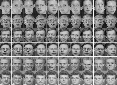
So the first thing we’ll need is some data to test our system. For now we’ll be skipping the facial detection part and using the AT&T Database of Faces (click this link for direct zip file download), which is a dataset containing ten pre-cropped pictures each for forty distinct individuals/subjects (400 pictures total). Just to make things a bit more interesting, there’s also some of the varying conditions we talked about present in some of the individuals pictures (e.g. people opening mouths and moving heads for different pictures, glasses on and off etc.).

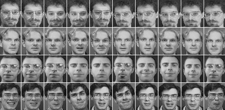
Sample faces from the dataset for four subjects.

To put together our supervised classification system, we’ll be using OpenCV (and its contrib modules, see pypi installation instructions). I’ll also be using matplotlib, numpy and pandas to examine our dataset and our results. I’m using Anaconda and writing my code in a python notebook (using jupyter notebook), but you could do this as a .py file in the IDE of your choice.

Loading the data set

Once you’ve downloaded and extracted the zip file, you’ll notice it contains a bunch of folders (s1-s40), each of these folders represents an individual person (or subject), and contains the ten cropped pictures of that persons face. First lets write a function to return a list of all the directories within a given path.

def list_dirs(basePath, ordered=True):
    """
        Return a list of all immediate sub-directories within basePath.
    """
    from os import listdir
    from os.path import isdir, join
    subDirs = [x for x in listdir(basePath) if isdir(join(basePath, x))]
    if ordered: subDirs.sort()
    return subDirs

Cool that’s ready to use, but we could also do with a function to return a list of full paths to the files within a given directory (the pictures of each subjects face).


def retrieve_file_paths(basePath, extension='.csv'):
    """
        Return a list of all files/paths to datasets from a given folder with a
        particular extension.
    """
    from os import listdir
    from os.path import splitext, isfile, join
    files = [x for x in listdir(basePath)
            if isfile(join(basePath, x)) and splitext(x)[1] == extension]

    # Return list of full paths
    paths = []
    for f in files:
        paths.append(basePath+f)
    return paths

Now we’re cooking, lets take a look at our dataset. So this next bit of code assumes that our extracted dataset folder “att_faces” is in the same directory as our python file or notebook, lets check out or list of directories, or subject IDs.


basePath = "att_faces/"

# Get list of subjects (each directory in this dataset represents a distinct subject)
subjectIDs = list_dirs(basePath)

subjectIDs

# Uncomment below if you're not using jupyter notebook
#print(subjectIDs)

Alright, that gave us a nice list of all of our subjects. Now we’re ready to load the dataset in to memory.


subjects = {}
for s in subjectIDs:
    # Fetch paths to all images for this subject
    imagePaths = retrieve_file_paths(basePath + s + '/', extension='.pgm')

    images = []
    for p in imagePaths:
        images.append(cv2.imread(p, 0))

    # Get integer value of subject ID
    sID = int(s.strip('s'))
    subjects[sID] = images

# This should print 40
print(len(subjects))

# Lets choose a subject
subject = subjects[6]
print('There are ', len(subject), 'images of this subject')

# Display random image
from matplotlib import pyplot as plt
plt.imshow(subject[6], cmap="gray")

# Use below instead of imshow if using another IDE
# plt.imsave('subject6Test.png', cmap="gray")

Having displayed or saved our image, you should be able to see this guy:

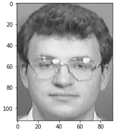
You may be wondering why we are using grayscale instead of colour images, this is because colour data doesn’t really help us identify facial features and tell faces apart. Going greyscale also drastically reduces the amount of data we’re storing for each image, which will really help the efficiency of our learning algorithm. Now our dataset is loaded in to memory, we’re ready to train our supervised machine learning algorithm.

Training and Testing the Recognizer

If you’re already familiar with training and testing supervised learning algorithms, you’ll know what’s coming. We need three things to train and evaluate a classifier or recognizer:

A set of training images – we’ll show these to our learning algorithm along with the subject labels, so our algorithm can learn/find the features that help identify a subject across their example training pictures.
A set of test images – these are images we’ll feed to the learning algorithm without subject labels after training, in the hope that our algorithm will accurately label the image. Of course we’ll need to keep track of the label somewhere else. This will help us evaluate performance along with…
A performance metric – some way to measure how well/accurately our system is working. This could be some function which produces a number which we’ll either want to increase (if its something like an accuracy measurement) or decrease (if its something like the number of incorrect guesses).

Generating our training and test sets should be pretty strait forward, we can just divide our existing set of images in to two sets, using one for training and the other for testing. The performance metric we’ll use will be the F1 score, I won’t go in to massive depth on the explanation or justification (that’s another article in its self), but very broadly it uses a combination of the precision and recall, which look at true and false positives and negatives from different perspectives to give a well rounded view of performance.

So here’s a question, how many examples should we use for training and how many should we use for testing? This is an interesting balance across many Machine Learning problems, too many samples training samples, and there may not be enough samples to thoroughly test performance, not enough training examples, and you may be in danger of overfitting your model. Overfitting is kind of the same as a student learning how to do a mock exam paper really well, but not being able to generalize when faced with a different unseen exam paper on the same subject (he/she should have looked at a wider variety of mock papers).

For finding the best balance, I propose a good old fashioned experiment. If we write some flexible functions, we should be able to easily experiment with different divisions of training and test data, so lets get to it!

First we’ll write a function to split our data set…

Both the training and testing sets should contain images of every subject, so for example we want to be able to train on 6 images of every subject and test on the remaining 4 images of each subject.

def train_test_split(dataset, numTrain):
    # Split testing and training data
    train = {}
    test = {}

    for sID, imageArr in dataset.items():
        train[sID] = imageArr[:numTrain]
        test[sID] = imageArr[numTrain:]

    return train, test

We’ll be using and training the OpenCV Local Binary Pattern (LBPH) Face Recognizer in this experiment. This handles feature extraction, comparison, and recognition for us. We’ll feed it greyscale images of our subjects, this object will then perform the feature extraction, producing LBPH vectors from the images, these vectors are then used in the comparison stage to produce our model. The model is then stored in the LBPH Recognizer class object internally, which is referred to when we pass in new unseen test images for the recognizer to label. There are a few alternatives for the feature extraction stage (insead of LBPH vectors), such as FisherFaces and Eigenfaces, but these are less robust when faced with changes in envrionmental conditions and noise (lighting, facial movements etc.). If you’re interested in reading more I left a link to the paper in the Links and Resources section.

For the purpose of flexibility and re-usability, we’ll write a function that takes an LBPH Recognizer object, a training set, and a test set, and returns a pandas data frame (table) containing the predicted label, actual label, and a confidence score for each prediction. We’ll also get the function to return us an F1 score, we’ll use sklearn to calculate our f1 score for us from our expected and predicted labels for each test item. The LBPH recognizer training and testing methods take a two lists as input, one list of numpy arrays representing our raw images, and a numpy array containing the subject label corresponding to each raw image, so we’ll write a function that formats our datasets to satisfy this requirement.

import pandas as pd
def format_dataset(dataset, shuffle=False):
    from random import shuffle as shuff

    images = []
    labels = []

    for label, imageArr in dataset.items():
        if shuffle: shuff(imageArr)
        for image in imageArr:
            labels.append(label)
            images.append(image)

    return labels, images

def run_evaluation(recognizer, trainSet, testSet):
    """
        Trains a LBPH classifier on the train set, evaluates it on the test set.
        Function returns a results table and a micro weighted F1 score.
    """

    from sklearn.metrics import f1_score

    trainLabels, trainImages = format_dataset(trainSet)
    testLabels, testImages = format_dataset(testSet)

    # Train the recognizer with the training set
    recognizer.train(trainImages, np.array(trainLabels))

    # Test the recognizer
    actualLabels = []
    predictedLabels = []
    predictionConfidence = []
    for label, imageArr in testSet.items():
        for img in imageArr:
            # Get tuple with predicted label and confidence value
            labConfTup = recognizer.predict(img)
            predictedLabels.append(labConfTup[0])
            predictionConfidence.append(labConfTup[1])
            actualLabels.append(label)

    # Create a results table from the data
    d = {'Predicted_Label': predictedLabels, 'Actual_Label':actualLabels,
         'Confidence':predictionConfidence}

    # Generate an f1 score
    f1 = f1_score(actualLabels, predictedLabels, average='micro')
    return pd.DataFrame(data=d), f1

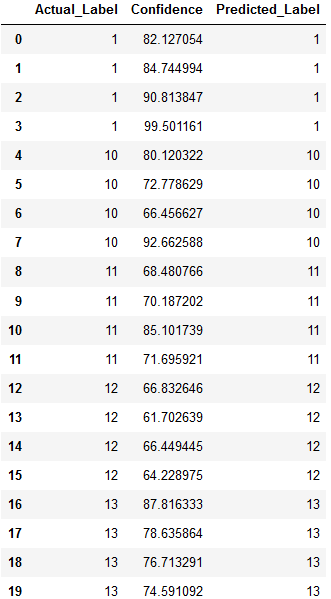
Hooray! Now comes the cool part, lets train and test our recognizer with our new function. I’m going to use 6 images of each subject for training, and 4 for testing.

# Create an OpenCV LBPHFaceRecognizer
recognizer = cv2.face.LBPHFaceRecognizer_create()

"""
    Split dataset, where 6 images will be used as training for each subject, and 4 will be used for testing.
"""
train, test = train_test_split(subjects, 6)

resTable, f1 = run_evaluation(recognizer, train, test)
# Use the below for jupyter notebook
resTable.head(20)
# Uncomment below for any other IDE
#print(resTable.head(20))

Looking at the first twenty predictions, with four images of each subject, it looks like our function is working as it should, and that our recognizer is working well.

Facial Recognition detailed results table

Now let’s check our F1-score.

f1 # Wrap this in a print function for another IDE

I got an F1-score of 0.9375, which is really good given that an F1 score of 1.0 would indicate perfect performance. The question is, can we do better? Here’s where our nifty function will come in quite handy. In this next experiment, we’ll run our train/test function in a for loop, incrementing the number of training images we use by one every iteration up to a total of 8, keeping a note of the sample size and f1 score.

# Lists to keep track of values at each iteration (these will be used to generate
# a graph later)
trainingSampleSize = []
f1Score = []

for trainSize in range(1, 8):
    # Create a fresh recognizer
    recognizer = cv2.face.LBPHFaceRecognizer_create()

    # Use a training set of size "trainSize"
    train, test = train_test_split(subjects, trainSize)
    # Evaluate the classifier
    resTable, f1 = run_evaluation(recognizer, train, test) 

    # Append data from this iteration to lists
    trainingSampleSize.append(trainSize)
    f1Score.append(f1)

# Create table of results
d = {'Training Samples':trainingSampleSize, 'F1 Score':f1Score}
df = pd.DataFrame(data=d)

df
# Uncomment below outside of jupyter notebook
# print(df.to_string())

The results are in!

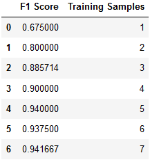
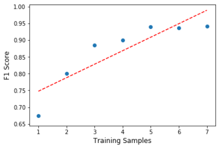
It looks like a 70-30 split on training and test data yielded the best results for me, not a huge improvement, but an improvement nonetheless. If we had more example images of each subject, it’s possible we could have seen a greater improvement in recognition using more than seven training samples. Lets also not forget that in our 70-30 split, there were less chances for our recognizer to get things wrong, which could have impacted our score.

Conclusion

In this tutorial, we took a high level overview of the facial recognition process and its stages, as well as the difference between supervised and unsupervised methods. We then covered some of the considerations to keep in mind when training a model, and wrote some functions to train and test a supervised LBPH Face Recognizer in python on the AT&T Database of faces, which achieved excellent performance with an F1 score of 0.94.

In the next articles we’ll explore and implement unsupervised methods that will let us recognize faces without training the model.

Something not quite right?

If you’ve spotted any mistakes or have any general feedback, please feel free to let me know in the comments below. Also if you think my code could be improved, go ahead and drop in a pull request on the github repository.